Essence of linear algebra
A geometric understanding of matrices, determinants, eigen-stuffs and more.
Vectors
- Always think vectors in the coordinate space
- It's a directed line, starting at the origin, with certain length
- Addition of vectors
- each vector represents a "movement" with steps and direction
- a sum of two vectors can be thought as a two-step movement: frist step move with vector 1 and move 2 after the first step move
- Vector multiple by a number ("scalar")
- "stretching" each coordinate by the value of scalar
Linear combinations, span, and basis vectors
- Span (of a vector): the line aligned with/goes through the vecor
Linear transformation and matrices
-
"Linear" transformation (properties) => grid lines remain parallel and evenly spaced:
- all lines remain as lines without getting curved
- the orgin remain fixed
- e.g. rotation, stretch
-
It can be considered as where the base vectors ($\hat{i}$ and $\hat{j}$) land after transformation, then everything else (i.e. all the vectors) in the coordinate follows
$$\text{if } \overrightarrow{v} = c_1 \hat{i} + c_2\hat{j}$$$$\text{and after transformation } \hat{i} \text{ lands on } \overrightarrow{i} \text{and } hat{j} \text{ lands on }\overrightarrow{j}$$$$\text{then transformed } \overrightarrow{v} \text{ can be written as } \text{if } \overrightarrow{v}' = c_1 \overrightarrow{i} + c_2\overrightarrow{j}$$- Thus the linear transformation of a 2-dimensional vector can be fully described by a $2 \times 2$ matrix defined by the vectors $\overrightarrow{i}$ and $\overrightarrow{j}$, or $[\overrightarrow{i} \ \overrightarrow{j}]$.
-
Calculation of linear transformation of a verction as the dot product of a matrix with a vector:
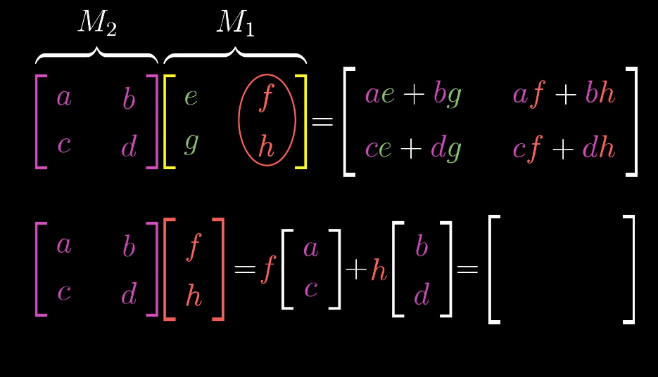
$$\begin{bmatrix} a & b \\ c & d \end{bmatrix} \begin{bmatrix} e \\ f \end{bmatrix} = e * \begin{bmatrix} a\\ c \end{bmatrix} + f * \begin{bmatrix} b \\ d \end{bmatrix} = \begin{bmatrix} a*e + b*f \\ c*e + d*f \end{bmatrix}$$- Matrices multiplication can be thought as splitting the second matrix conlumn-wise into individual column vectors, conduct above calculation for each column vector and combine the results column-wise.
-
Special linear transformation:
-
Shear, whose transformation matrix is
$$\begin{bmatrix} 1 & 1 \\ 0 & 1\end{bmatrix} $$ -
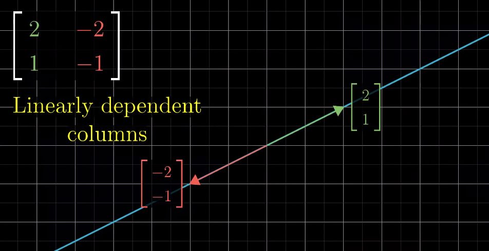
Linearly dependent transformation: the resulting transformed spaced is squashed into a 1-dimensional line
-
Matrix multiplication as composition
-
Multiplicaiton of two matrices ==> two-step transformation (composition) of the space geometrically
-
This is basically what I summarized in linear transformation:
-
This indicates that the order of the matrices multiplication matters, i.e. change the order of matrices will change the result
-
To compute the determinant
$$\det\left(\begin{bmatrix} a & b \\ c & d\end{bmatrix} \right) = ad - bc$$
Three-dimensional linear transformation
- Very similar to two-dimensional transformation
- Instead of move/transform the $x-$ and $y-$ cordinates, there is just an additional $z-$axis to be transformed
The determinant
-
Geometric explanation: the "scaling" factor a linear transformation imposes to the area (2D) or volume (3D or above) defined by the basis factors (since the area defined by the basis vectors is 1, the deteriminant is actually the signed area of the space defined by the column vectors in the transformation matrix)
-
Determinant can be negative, depending on the orientation of the transformation (negative if orientation is inverted/flipped)
-
Determinant of zero meaning the transformation leads to 0 scaling to the area/volume or even to a single point; it also corresponds to linearly dependent transformation
-
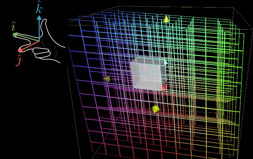
Right-hand rule: to check the orientation of the transformation in 3D
Inverse matrices, column space and null space
- Linear system of equations <=> matrix, vector product => linear transformation of a vector
- Inverse of a matrix => a back transformation corresponds to the matrix itself
- The inverse of a matrix exists as long as its determinant is non-zero; in contrast, if the determinant is 0, the inverse doesn't exist, i.e. we can expand a lower dimension space to a higher dimension one. There can be infinite possible higher dimensional space corresponds to the lower space in such case.
- In some special cases, when the determinant is 0, there may still be solutions to some vectors, when the output verctors are those lie along the lower dimension line/space after the transformation (why??)
- Rank:
- geometrically, it's the number of dimensions of the resulting space/output after a linear transformation, e.g. if the transformation leads to a line, then the rank of the transformation matrix is 1;
- Linear algebra: linearly independent columns of the transformation matrix
- Column space of a matrix: set of all possible outputs of the linear transformation <=> the # of spans of colums of the transformation matrix
- Ranks of a matrix is the number of dimensions in its column space; $\begin{bmatrix}0\\0\end{bmatrix}$ is always in the column space
- Full rank: when the rank is as high as it can be;
- for a full rank transformation, only the original can lands on itself;
- for a non-full rank transformation, there are infinite numbers of vectors can land on the origin; it is a whole line of vectors in 2D cases or whole planeful of vectors get squished into the original in 3D cases (that the # of deminsions lost in the transformation).
- Null space: the set of vectors that lands on the original or the kernel of the matrix
Nonsqure matrices transformations between dimensions
- Columns of the matrix stands for the number of basis vectors (in input)
- Rows of the matrix stands for the number of coordinates of each landing spots (in output)
Dot products and duality
-
Geometrical interpretation
- Project one vector to the other vector, multiple the projected vector's length with the length of the other vector
-
Numerical calculation
$$\begin{bmatrix} a \\ b \end{bmatrix}\cdot \begin{bmatrix} c \\ d \end{bmatrix} = [a \ b] * \begin{bmatrix} c \\ d \end{bmatrix} = a*c + b*d$$ -
Connection between geometric interpretation and linear transformation of a vector
- Dot product is equivalent to matrix, vector multiplcation, i.e. a $1\times 2$ matrix/vector times a $2\times 1$ vector
- This matrix/vector multiplication is connected with the linear transformation of the vector, which, geometically speaking, projects/transforms a vector to a one-dimensional line (this line is defined by the other vector in the dot product)
-
Note: [other vector products](./Note-#Miscellaneous Notes.md)
Cross products (of two vectors, $\vec{v} \times \vec{w}$)
-
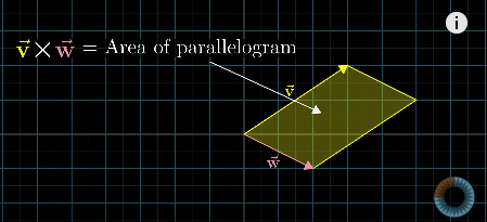
Geometric interpretation: Area of the parallelogram formed by two vectors (in two dimensional space)
- If $\vec{v}$ is on the right of $\vec{w}$, the product is positive; otherwise, the product is negative.
- $\vec{v} \times \vec{w} = -\vec{w} \times \vec{v}$
-
Numeric calculation
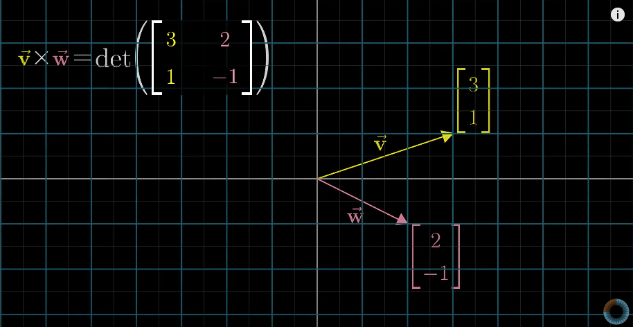
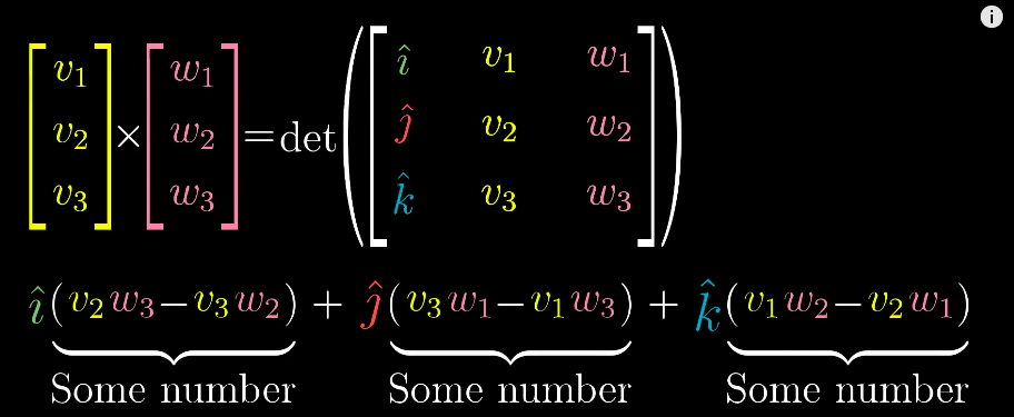
-
But the actual results of a cross product of two vectors is actually another vector, which is perpendicular to the parallelogram with length equals to the area of the parallelogram and direction is decided by the "right-hand rule"
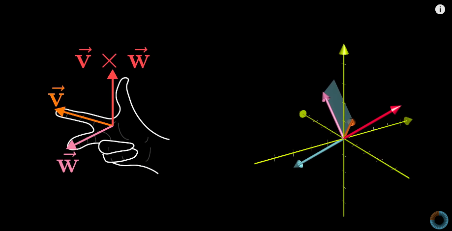
Cross products in the light of linear transformations
Cramer's rule, explained geometrically
-
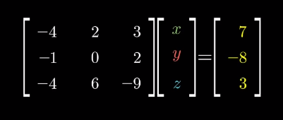
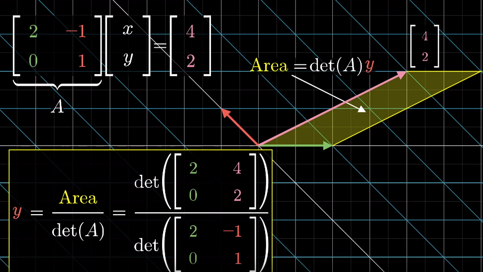
The solution to the system of equations is givcen by the Cramer's rule:

-
Derivation of Cramer's rule
-
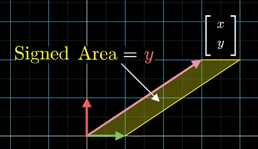
Any vector $\overrightarrow{y}$ (e.g. $\begin{bmatrix}x\\y\end{bmatrix}$) can define a signed area (2D) or a "volume" (3D or above) with the basis vectors and the area/volume can be expressed by the coordinate of x or y axis
-
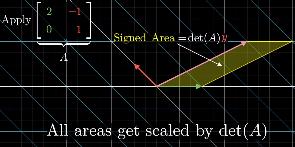
When applying a linear transformation to the vector, above area/volume is scaled by the determinant of the transformation matrix
-
The resulting vector also defines an area/volume, which can be calculated as the determinant of a matrix based on the transformation matrix and replacing one of its column by the resulting vector (which one to replace is depnent on which basis vector the original area is calculated from)
-
Change of basis
Eigenvectors and eigenvalues
-
Many vectors get knoced out their spans after linear transformation, but some do remain on their spans (meaning only stretch or squish effect is applied to them)
-
Those special vectors that remain on their span after linear transformation are eigenvectors of the transformation
-
Eigenvalues are just the factors that define how much stretch/squish is applied to the eigenvectors in the linear transformation
$$A\overrightarrow{v} = \lambda\overrightarrow{v}$$where $\overrightarrow{v}$ is the eigenvector of tranformation $A$ and $\lambda$ is the eigenvalue corresponds to the eigenvector
- How to solve above equation?
-
It can be thought as in the linear transformation, all the base vectors are multipled by a constant $\lambda$:
$$\lambda \mathbb{I}$$ -
Then the euqation becomes
$$A\overrightarrow{v} = \lambda\mathbb{I}\overrightarrow{v}$$$$(A - \lambda\mathbb{I}) \overrightarrow{v} = \overrightarrow{0}$$ -
This leads to the fact that
$$\det(A - \lambda\mathbb{I}) = 0$$
-
- How to solve above equation?
-
-
Geometric application: 3D rotation. The eigenvector is the axis of rotation
-
Some transformations may have more than one eignevector/eigenvalue but some may have no eigenvector/eigenvalue, e.g. roration in 2D space
-
It's also possible that a single eigenvalue has more than a single eigenvectors, it can have a line full of eigenvectors, e.g. in Shear transformation the eigen value is 1 and all the vectors on the x-axis are it's eigenvectors or a transformation that scales the space by a constant, there is only one eigenvalue but infinite numbers of eigenvectors
-
Eigenbasis: the basis vectors are the also eigenvectors of the linear transformation.
-
It comes with the transformation with diagonal matrices, where the diagonal values are the eigenvalues.
-
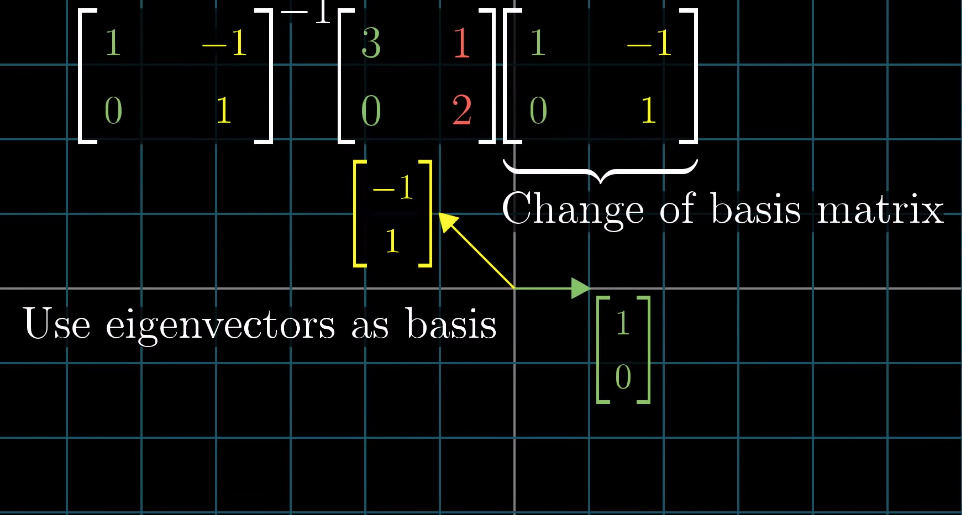
What if the original basis vectors are not eigenvectos? Change the coordinate system so that the eigenvectors become basis vectors.
- make those eigenvectors as colums of a matrix, known as the change of basis matrix,
- sandwich the original transformation matrix with the inverse of the change of basis matrix and itsel: the result will be the same transformation but using the new coordinate system and this (sandwich) matrix is guaranteed to be diagonal
- The column in the resulsting diagnoal matrix are the eigenbasis
-
This trick can be used to calculate the nth power of a matrix that is not diagonal
-
NOTE: this manipulation is not always feasible, when the existing eigenvectors are not enough to span the entire/full space then it's not feasible
-