[book] Causal inference in statistics a primer
a study note of [1]
Chapter 1 Preliminaries: Statistical and Causal Models
Simpson's Paradox
The paradox refers to the existence of data in which a statistical association that holds for an entire popu- lation is reversed in every subpopulation.
Example 1

The first row shows the outcome for male patients; the second row shows the outcome for female patients; and the third row shows the outcome for all patients, regardless of gender. In male patients, drug takers had a better recovery rate than those who went without the drug (93% vs 87%). In female patients, again, those who took the drug had a better recovery rate than nontakers (73% vs 69%). However, in the combined population, those who did not take the drug had a better recovery rate than those who did (83% vs 78%).
Explaination:
As we can see from the data, women are significantly more likely to take the drug than men are (i.e. there is gender imbalance in the two treatment arm). So, the reason the drug appears to be harmful overall is that, if we select a drug user at random, that person is more likely to be a woman and hence less likely to recover than a random person who does not take the drug. Put differently, being a woman is a common cause of both drug taking and failure to recover. Therefore, to assess the effectiveness, we need to compare subjects of the same gender (i.e. control for gender), thereby ensuring that any difference in recovery rates between those who take the drug and those who do not is not ascribable to estrogen.
Example 2

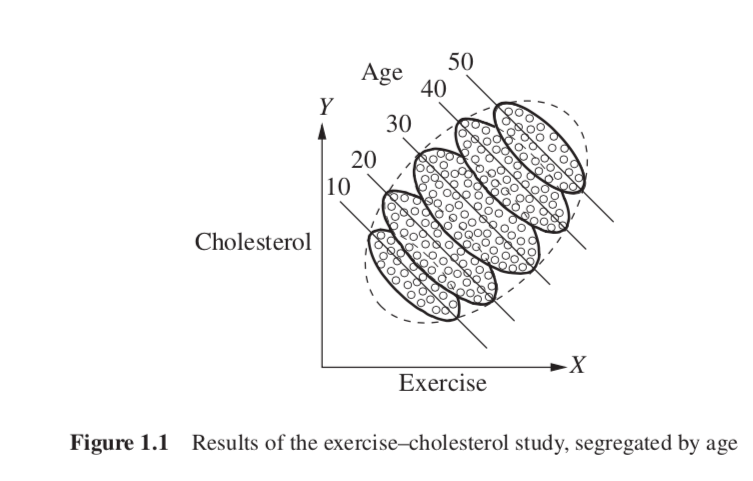
We see that there is a general trend downward in each group; the more young people exercise, the lower their cholesterol is, and the same applies for middle-aged people and the elderly.

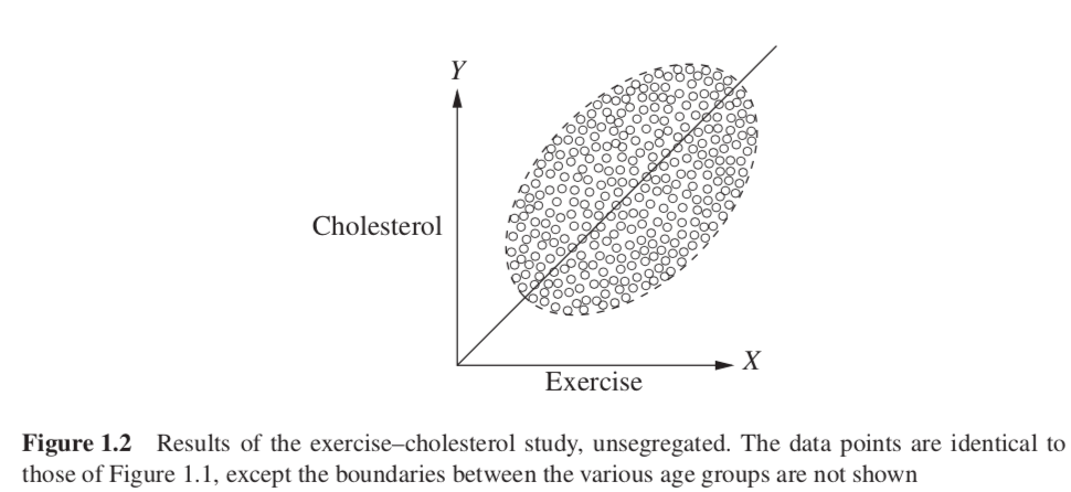
However, we use the same scatter plot, but we don’t segregate by gender (as in Figure 1.2), we see a general trend upward; the more a person exercises, the higher their cholesterol is.
Explaination:
Older people, who are more likely to exercise (Figure 1.1), are also more likely to have high cholesterol regardless of exercise, then the reversal is easily explained, and easily resolved. Age is a common cause of both treatment (exercise) and outcome (cholesterol). So we should look at the age-segregated data in order to compare same-age people and thereby eliminate the possibility that the high exercisers in each group we examine are more likely to have high cholesterol due to their age, and not due to exercising.
Example 3 (segregated data doesn't give correct answer)

we looked at the same numbers from our first example of drug taking and recovery, instead of recording participants’ gender, patients’ blood pressure were recorded at the end of the experiment. In this case, we know that the drug affects recovery by lowering the blood pressure of those who take it—but unfortunately, it also has a toxic effect. At the end of our experiment, we receive the results shown in Table 1.2. (Table 1.2 is numerically identical to Table 1.1, with the exception of the column labels, which have been switched.)
Explaination:
In the general population, the drug might improve recovery rates because of its effect on blood pressure. But in the subpopulations—the group of people whose posttreatment BP is high and the group whose posttreatment BP is low—we, of course, would not see that effect; we would only see the drug’s toxic effect. Treatment --> blood pressure --> outcome, conditional on blood pressure will remove the treatment effect on the outcome
-
There is, in fact, no way to represent any causal information in contingency tables (such as Tables 1.1 and 1.2), on which statistical inference is often based. (why? is it because contingency tables can only represent association instead of causation?)
-
In order to rigorously approach our understanding of the causal story behind data, we need four things:
- A working definition of “causation.” (A variable X is a cause of a variable Y if Y in any way relies on X for its value. or X is a cause of Y if Y listens to X and decides its value in response to what it hears.)
- A method by which to formally articulate causal assumptions—that is, to create causal models.
- A method by which to link the structure of a causal model to features of data.
- A method by which to draw conclusions from the combination of causal assumptions embedded in a model and data.
Chapter 2 Graphical Models and Their Applications
Chapter 3 The Effects of Interventions
3.1 Interventions
- When we intervene on a variable in a model, we fix its value. We change the system, and the values of other variables often change as a result. When we condition on a variable, we change nothing; we merely narrow our focus to the subset of cases in which the variable takes the value we are interested in.
- When we intervene to fix the value of a variable, we curtail the natural tendency of that variable to vary in response to other variables in nature. This amounts to performing a kind of surgery on the graphical model, removing all edges directed into that variable.
- Intervening on a variable results in a totally different pattern of dependencies than conditioning on a variable. Moreover, the latter can be obtained directly from the data set; while the former varies depending on the structure of the causal graph.
- In notation, we distinguish between cases where a variable $X$ takes a value $x$ naturally and cases where we fix $X = x$ by denoting the latter $do(X = x)$. So $P(Y = y|X = x)$ is the probability that $Y = y$ conditional on finding $X = x$, while $P(Y = y|do(X = x))$ is the probability that $Y = y$ when we intervene to make $X = x$.
- In the distributional terminology, $P(Y = y|X = x)$ reflects the population distribution of $Y$ among individuals whose $X$ value is $x$. On the other hand, $P(Y = y|do(X = x))$ represents the population distribution of $Y$ if everyone in the population had their $X$ value fixed at $x$. We similarly write $P(Y = y|do(X = x), Z = z)$ to denote the conditional probability of $Y = y$, given $Z = z$, in the distribution created by the intervention $do(X = x)$.
- It is worth noting here that we are making a tacit assumption here that the intervention has no “side effects,” that is, that assigning the value $x$ for the valuable $X$ for an individual does not alter subsequent variables in a direct way.
3.2 The Adjustment Formula
-
Denoting the first intervention by $do(X = 1)$ and the second by $do(X = 0)$, our task is to estimate the difference $$P(Y = 1|do(X = 1)) − P(Y = 1|do(X = 0))$$ which is known as the “causal effect difference,” or “average causal effect” (ACE).
-
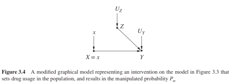
The causal effect $P(Y = y|do(X = x))$ is equal to the conditional probability $P_m(Y = y|X = x)$ that prevails in the manipulated model of Figure 3.4.

-
the marginal probability $P(Z = z)$ is invariant under the intervention, because the process determining $Z$ is not affected by removing the arrow from $Z$ to $X$.
-
the conditional probability $P(Y = y|Z = z, X = x)$ is invariant, because the process by which $Y$ responds to $X$ and $Z, Y = f (x, z, u_Y )$, remains the same, regardless of whether $X$ changes spontaneously or by deliberate manipulation. We can therefore write two equations of invariance: $$P_m(Y=y|Z=z,X=x)=P(Y=y|Z=z,X=x) \text{ and } P_m(Z=z)=P(Z=z)$$
-
using the invariance relations, we obtain a formula for the causal effect, in terms of preintervention probabilities:
$$ \begin{align} P(Y = y|do(X = x)) & = P_m(Y = y|X = x)\\ & = \sum_z P_m(Y = y|X = x,Z = z)P_m(Z = z|X = x)\\ & = \sum_z P_m(Y = y|X = x,Z = z)P_m(Z = z)\\ & = \sum_z P(Y = y|X = x, Z = z)P(Z = z) \end{align} $$- This is called the adjustment formula, it computes the association between X and $Y$ for each value $z$ of $Z$, then averages over those values. This procedure is referred to as “adjusting for $Z$” or “controlling for $Z$".
- No adjustment is needed in a randomized controlled experiment since, in such a setting, the data are generated by a model which already possesses the structure of Figure 3.4, hence, $P_m = P$ regardless of any factors $Z$ that affect $Y$.
- In practice, investigators use adjustments in randomized experiments as well, for the purpose of minimizing sampling variations (Cox 1958)
-
The graph of Figure 3.5 shows no arrow entering X, since X has no parents. This means that no surgery is required; the conditions under which data were obtained were such that treatment was assigned “as if randomized.” If there was a factor that would make subjects prefer or reject treatment, such a factor should show up in the model; the absence of such a factor gives us the license to treat X as a randomized treatment.

-
Under such conditions, the intervention graph is equal to the original graph—no arrow need be removed—and the adjustment formula reduces to
$$P(Y = y|do(X = x)) = P(Y = y|X = x)$$
-
-
3.2.1 To Adjust or not to Adjust
-
The Causal Effect Rule: Given a graph G in which a set of variables PA are designated as the parents of $X$, the causal effect of $X$ on $Y$ is given by
\begin{align} P(Y = y| do(X = x)) & = \sum_z P(Y = y | X = x, PA = z) P(PA = z)\ & = \sum_z \frac{P(Y = y | X = x, PA = z) P(PA = z) * P(X=x|PA = z)}{P(X=x|PA = z)}\ & = \sum_z \frac{P(Y = y, X = x, PA = z)}{P(X=x|PA = z)} \end{align}
where $z$ ranges over all the combinations of values that the variables in PA can take and $P(X=x|PA = z)$ is the propensity score.
3.2.2 Multiple Interventions and the Truncated Product Rule
\begin{align} P(x, y, z) & = P(z)P(x|z)P(y|x, z)\ P(z, y|do(x)) & = P_m(z)P_m(y|x, z) = P(z)P(y|x, z)\ \Rightarrow P(z, y|do(x)) & = \frac{P(x, y, z)}{P(x|z)} \end{align}
- It tells us that the conditional probability $P(x|z)$ is all we need to know in order to predict the effect of an intervention $do(x)$ from nonexperimental data governed by the distribution $P(x, y, z)$.
3.3 The Backdoor Criterion
-
Challenge: variables may have unmeasured parents that, though represented in the graph, may be inaccessible for measurement. In those cases, we need to find an alternative set of variables to adjust for.
-
Question: Under what conditions does a causal story permit us to compute the causal effect of one variable on another, from data obtained by passive observations, with no interventions? (Under what conditions, is the structure of the causal graph sufficient for computing a causal effect from a given data set?)
-
Solution: one of the most important tools we use to determine whether we can compute a causal effect is a simple test called the backdoor criterion. Using it, we can determine whether, for any two variables $X$ and $Y$ in a causal model represented by a DAG, which set of variables $Z$ in that model should be conditioned on when searching for the causal relationship between $X$ and $Y$.
-
Definition (The Backdoor Criterion): Given an ordered pair of variables $(X, Y)$ in a directed acyclic graph $G$, a set of variables $Z$ satisfies the backdoor criterion relative to $(X, Y)$ if no node in $Z$ is a descendant of $X$, and $Z$ blocks every path between $X$ and $Y$ that contains an arrow into $X$.
-
If a set of variables $Z$ satisfies the backdoor criterion for $X$ and $Y$, then the causal effect of $X$ on $Y$ is given by the formula
-
When trying to find the causal effect of $X$ on $Y$, we want the nodes we condition on to block any “backdoor” path in which one end has an arrow into $X$, because such paths may make $X$ and $Y$ dependent, but are obviously not transmitting causal influences from $X$, and if we do not block them, they will confound the effect that $X$ has on $Y$.
-
Consider the fact that $P(Y = y|do(X = x))$ is an empirical fact of nature, not a byproduct of our analysis. That means that any suitable variable or set of variables that we adjust on—whether it be $PA(X)$ or any other set that conforms to the backdoor criterion—must return the same result for $P(Y = y|do(X = x))$. In the case we looked at in Figure 3.6 ($Y \leftarrow X \leftarrow Z \rightarrow W \rightarrow Y$), this means that
\begin{align} && \sum_w P(Y = y|X = x,W = w)P(W = w) \ && = \sum_z P(Y = y|X = x, Z = z)P(Z = z) \end{align}
- In the cases where we have multiple observed sets of variables suitable for adjustment (e.g., in Figure 3.6, if both W and Z had been observed), it provides us with a choice of which variables to adjust for.
- The equality constitutes a testable constraint on the data when all the adjustment variables are observed, much like the rules of $d$-separation.
-
3.4 The Front-Door Criterion
-
Problem: The backdoor criterion provides us with a simple method of identifying sets of covariates that should be adjusted for when we seek to estimate causal effects from nonexperimental data. It does not, however, exhaust all ways of estimating such effects. The $do$-operator can be applied to graphical patterns that do not satisfy the backdoor criterion to identify effects that on first sight seem to be beyond one’s reach.
-
The front-door formula
\begin{align} P(Y =y | do(X = x)) = \ \sum_z\sum_x' P(Y = y | Z = z, X = x') P(X = x') P(Z = z|X = x) \end{align}
-
Definition (Front-Door) A set of variables $Z$ is said to satisfy the front-door criterion relative to an ordered pair of variables $(X, Y)$ if
- $Z$ intercepts all directed paths from $X$ to $Y$.
- There is no unblocked path from $X$ to $Z$.
- All backdoor paths from $Z$ to $Y$ are blocked by $X$.
-
Theorem (Front-Door Adjustment) If $Z$ satisfies the front-door criterion relative to $(X, Y)$ and if $P(x, z) > 0$, then the causal effect of $X$ on $Y$ is identifiable and is given by the formula
$$P(y|do(x)) = \sum_z P(z|x) \sum_{x′} P(y|x′, z)P(x′)$$
3.5 Conditional Interventions and Covariate-Specific Effects
3.6 Inverse Probability Weighing
3.7 Mediation
3.8 Causual Inference in Linear Systems
3.8.1 Structual vesus Regression Coefficients
3.8.2 The Causal Interpretation of Structural Coefficients
3.8.3 Indentifying Structural Coefficients and Causal Effect
3.8.4 Mediation in Linear Systems
References
Pearl, Judea and Glymour, Madelyn and Jewell, Nicholas P (2016). Causal inference in statistics: A primer. ↩︎