[book] Regression Modeling Strategies
A reading note of [1]
Chapter 9 Overview of Maximum Likelihood Estimation
- How to understand Fisher information and what info it provides: The degree of peakedness of a function at a given point is the speed with which the slope is changing at that point, that is, the slope of the slope or second derivative of the funciton at that point.
- i.e. at the peak of a function, the speed of slope change is the slowest
- An estimate of variance is given by the inverse of the information at the point estimate (e.g. the MLE)
2. Hypothesis testing
2.1 Likelihood ratio test
-
This test statistic is the ratio of the likelihood at the hypothesized parameter values to the likelihood of the data at the maximum (i.e., at parameter values = MLEs).
- −2× the log of this likelihood ratio has desirable statistical properties.
for large enough sample size, where $p$ is the number parameters to be tested
2.2 Wald test
-
The Wald test statistic is a generalization of a t- or z- statistic. It is a function of the difference in the MLE and its hypothesized value, normalized by an estimate of the standard deviation of the MLE. For large enough $n$,
$$W = \frac{(\hat{\theta} - \theta_0)^2}{var(\hat{\theta})}\sim \chi^2_p$$
- Variance of MLE is the inverse of the oberved Fisher information $1/I(\hat{\theta})$
- $\sqrt{W}$ can follow either $t$ or normal distribution, depending on if the variance of the estimate is an estimated (like in the normal data) or not (like in the binary data)
2.3 Score test
- Rao’s score statistic measures how far from zero the score function is when evaluated at the null hypothesis.
- If the MLE happens to equal the hypothesized value $\theta_0$, $\theta_0$ maximizes the likelihood and so $U(\theta_0) = 0$.
- The variance of the score function is the Fisher information $I(\theta_0)$
- Test statistic for score test is defined as $\frac{U(\theta_0)^2}{I(\theta_0)} \sim \chi^2_p$
- Thus the score test doesn't invole estimating the MLE
Which test to use when

3. General case
-
Estimating a vector of parameters
-
Score vector: first derivative of the log likelihood function w.r.t. all the parameters
$U(B) = (\partial/\partial B)\log L(B)$
-
Fisher information matrix: a $p\times p$ matrix whose elements are the negative of the expectation of all second partial derivatives of $\log L(B)$
$I^*(B) = -E(\partial^2/\partial B\partial B')\log L(B)$
-
Observed information matrix: is the information matrix without taking expectation
$I(B) = -(\partial^2/\partial B\partial B')\log L(B)$
-
-
Global test statistics
- The extention from one dimentional test to $p-$dimensional test
-
Testing a subset of the parameters
-
Tests based on contrasts
6. Confidence intervals
8. Further use of the log likelihood
9. Weighted maximum likelihood estimation
10. Penalized maximum likelihood estimation
Chapter 13 Ordinal Logistic Regression
1. Background
2. Ordinality assumption
3. Proportional odds model
3.1 Model
3.2 Assumptions and interpretation of parameters
3.3 Estimation
3.4 Residuals
-
In binary logistic regression, partial residuals are very useful as they allow the analyst to fit linear effect for all the predictors but then to nonparametrically estimate the true transformation that each predictor requires.
$$ r_{im} = \hat{\beta}_mX_{im} + \frac{Y_i - \hat{P}_i}{\hat{P}_i(1-\hat{P}_i)} $$ where
$$ \hat{P}_i= \frac{1}{1 +\exp[-(\alpha + X_i\hat{\beta})]} $$- A smoothed plot (e.g., using the moving linear regression algorithm in
loess) of $X_{im}$ against $r_{im}$ provides a nonparametric estimation of how $X_m$ relates to the log relative odds that $Y = 1 | X_{m}$. - Since partial residuals allow examination of predictor transformations (linearity) while simultaneously allowing examination of PO (parallelism), partial residual plots are generally preferred over score residual plots for ordinal models.
- A smoothed plot (e.g., using the moving linear regression algorithm in
3.5 Assessment of model fit
-
Score test in
PROC LOGISTIC: extreme anti-conservatism in many cases -
Compare means of $X|Y$ with and without assuming PO
-
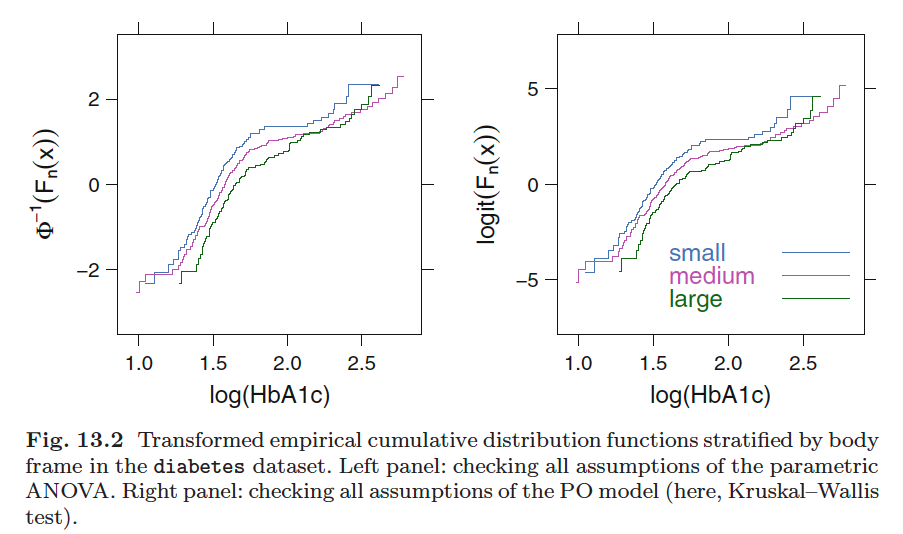
Stratifying one each predictor and computing the logits of all proportions of the form $Y\ge j, j = \text{1, 2, }\cdots, k$. When proportional odds holds, the difference in logits between different values of $j$ should be the same at all levels of $X$, because the model dictates that $logit(Y\ge j| X) - logit(Y\ge i|X) = \alpha_j - \alpha_i$, for any constant $X$.
-
We check both the consistency of $logit(Y\ge j| X) - logit(Y\ge i|X)$ at different $X$ levels
-
Or we can check the parallelism of $logit(Y\ge j| X) - logit(Y\ge j|X+k)$ for $Y = 1, \cdots, J$ (right below)

-
-
Regarding assessment of linearity and additivity assumptions, splines, partial residual plots, and interaction tests are among the best tools.
3.6 Quantifying predictive ability
- $R_N^2$ coefficient: model LR $\chi^2$ ($\chi^2$ added to a model containing only the $k$ intercept parameter)
- Somers’ $D_{xy}$ rank correlation between $X\hat{\beta}$ and $Y$
- Probability of concordance $c$ (a generalized ROC area): the fraction of pairs for which the values of $X\hat{\beta}$ are in the same direction among all possible pairs of subjects having different $Y$ values
- $D_{xy} = 2(c - 0.5)$
3.7 Describing the fitted model
- $logit(Y\ge j|X)$, the linear predictor
- $Prob(Y\ge j| X)$
- $Prob(Y=j|X)$
- Quantiles of $Y|X$, e.g. the median
- $E(Y|X)$ if $Y$ is interval scaled
3.8 Validating the fitted model
- The PO model is validated much the same way as the binary logistic model
- For estimating an overfitting-corrected calibration curve one estimates $Pr(Y ≥ j|X)$ using one $j$ at a time.
3.9 R function
{rms}:rms::lrm: intended to be used for the cases where the number of unique values of $Y$ are less than a few dozerms::orm: handles the continuous Y case efficiently and allows for links other than the logit
{Hmisc}:popowerandposamsizecompute power and sample size estimates for ordinal responses using the proportional odds model.
4. Continuation ratio model
4.1 Model
-
The continuation ratio (CR) model is based on conditional probabilities. The (forward) CR model is defined as follows:
\begin{align} P(Y=j|Y\ge j, X) & = \frac{1}{1+\exp[-(\theta_j + X\gamma)]}\ logit(Y=0|Y\ge0, X) & = logit(Y=0|X)\ &=\theta_0 + X\gamma\
logit(Y = k-1|Y \ge k-1, X) & = \theta_{k-1} + X\gamma \end{align}
- the CR model has been said to be likely to fit ordinal responses when subjects have to “pass through” one category to get to the next.
- It is a discrete version of the Cox PH model, the discrete hazard function is defined as $P(Y=j|Y\ge j)$.
Chapter 20 Cox Proportional Hazards Regression Model
1. Model
1.7 Extending the (PH Cox) model by stratification
-
The model assumes different baseline hazard but common regression coefficient among stratified models
$\lambda(t | C =j) = \lambda_j(t)\exp(X\beta)$
- The idea is to allow the form of the underlying hazard function to vary across levels of the stratification factors
-
In most cases the loss of efficiency by stratification is small as long as the number of strata is not too large with regard to the total number of events.
- A stratum that contains no events contributes no information to the analysis, so such a situation should be avoided if possible.
-
If different strata are made up of independent subjects, the strata are independent and the likelihood functions are multiplied together to form a joint likelihood over strata. Log likelihood functions are thus added over strata.
- No inference can be made about the stratification factors. They are merely “adjusted for.”
-
Stratification is useful for checking the PH and linearity assumptions for one or more predictors.
- Predicted Cox survival curves can be derived by modeling the predictors in the usual way, and then stratified survival curves can be estimated by using those predictors as stratification factors.
- Other factors for which PH is assumed can be modeled in both instances.
- By comparing the modeled versus stratified survival estimates, a graphical check of the assumptions can be made.
-
Besides allowing a factor to be adjusted for without modeling its effect a stratified Cox PH model can also allow a modeled factor to interact with strata:
$\lambda(t|X_1, C=j) = \lambda_j(t)\exp(\beta_1X_1 + \beta_2X_2)$ for $j = 1, 2$ (example)
where $X_2 = 0$ for $j = 1$ and $X_1$ for $j=2$
-
The stratified Cox model turns out to be a generalization of the conditional logistic model for analyzing matched set (e.g., case-control) data. (??)
- Each stratum represents a set, and the number of “failures” in the set is the number of “cases” in that set.
- For $r : 1$ matching ($r$ may vary across sets), the Breslow likelihood may be used to fit the conditional logistic model exactly. For $r : m$ matching, an exact Cox likelihood must be computed.
3. Sample size considerations
-
Then the Kaplan-Meier estimate (one-sample) is just one minus the empirical cumulative distribution function, assuming there is no censoring. By the Dvoretzky-Kiefer-Wolfowitz inequality, the maximum absolute error in an empirical distribution function estimate of the true continuous distribution function is less than or equal to $\epsilon$ with probability of at least $1 − 2e^{−2n\epsilon^2}$.
-
To estimate the subject-specific survival curves $(S(t|X))$ will require greater sample sizes, as will having censored data.
-
To estimate hazard ratio:
-
if the total sample size is $n$ and the number of events in the two categories are respectively $e_0$ and $e_1$, the variance of the log hazard ratio is approximately $v = \frac{1}{e_0} + \frac{1}{e_1}$
-
Letting $z$ denote the $1 − \alpha/2$ standard normal critical value, the multiplicative margin
of error (MMOE) with confidence $1 − \alpha$ is given by $\exp(z\sqrt{v})$.
-
4. Test statistics
- Wald, score, and likelihood ratio statistics are useful and valid for drawing inferences about β in the Cox model.
- If there is a single binary predictor in the model that describes two groups, the score test for assessing the importance of the binary predictor is virtually identical to the Mantel–Haenszel log-rank test for comparing the two groups.
- If the analysis is stratified for other (nonmodeled) factors, the score test from a stratified Cox model is equivalent to the corresponding stratified log-rank test.
- The likelihood ratio or Wald tests could also be used in this situation, and in fact the likelihood ratio test may be better than the score test (i.e., type I errors by treating the likelihood ratio test statistic as having a $\chi^2$ distribution may be more accurate than using the log-rank statistic).
- The Cox model can be thought of as a generalization of the log-rank procedure since it allows one to test continuous predictors, perform simultaneous tests of various predictors, and adjust for other continuous factors without grouping them. Although a stratified log-rank test does not make assumptions regarding the effect of the adjustment (stratifying) factors, it makes the same assumption (i.e., PH) as the Cox model regarding the treatment effect for the statistical test of no difference in survival between groups.
5. Residuals
-
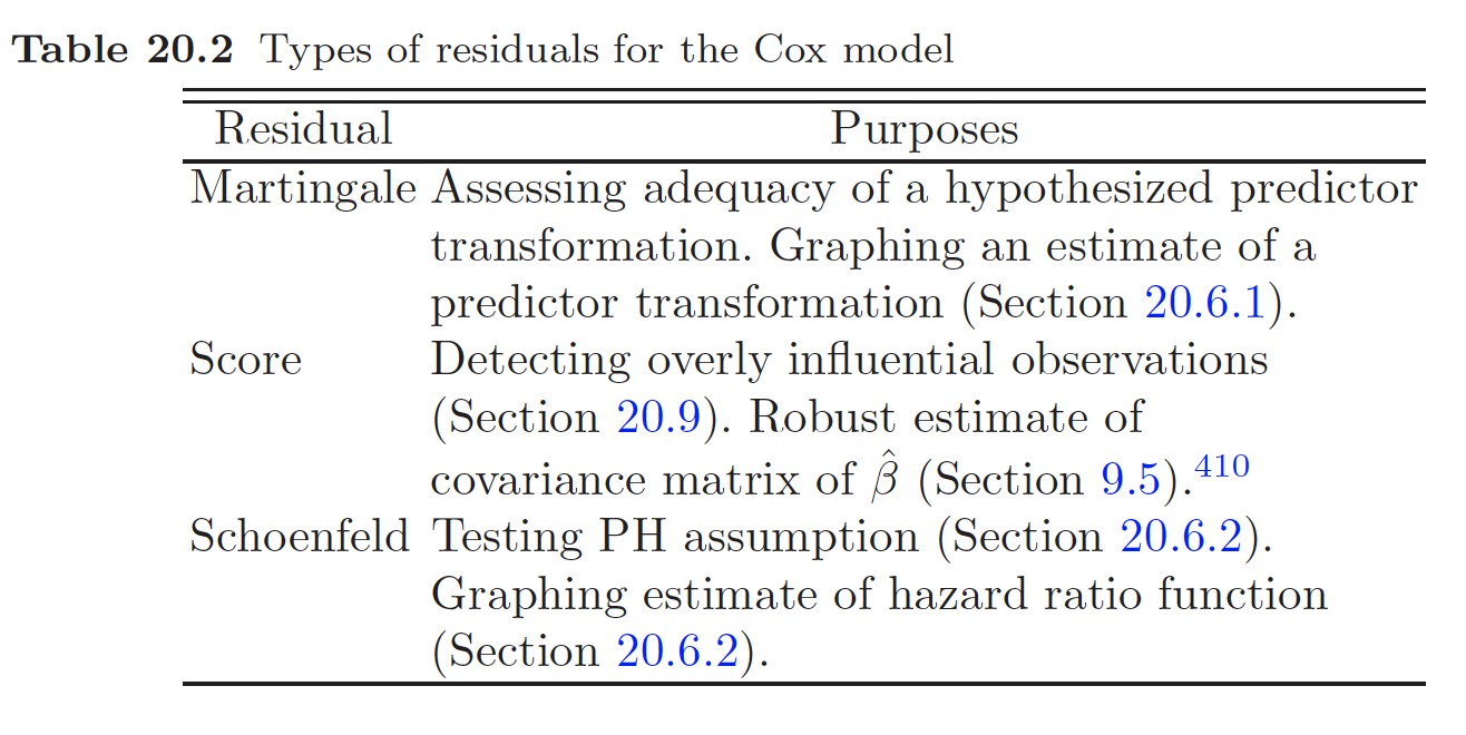
Therneau et al. discussed four types of residuals from the Cox model**: martingale, score, Schoenfeld**, and deviance.

6. Assessment of model fit
7. What to do when PH fails
- Also check note on Cox PH Model
References
Harrell, Frank E (2017). Regression modeling strategies. ↩︎