Cox PH model
Assumptions
Though the Cox model is non-parametric to the extent that no assumptions are made about form of the baseline hazard, there are still a number of important issues which need be assessed before the model results can be safely applied.
-
Non-informative censoring: the mechanisms giving rise to censoring of individual subjects are not related to the probability of an event occurring.
-
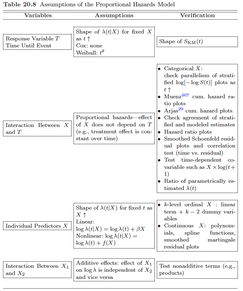
Proportional hazards. In a regression type of setting this means that the survival curves for two strata (determined by the particular choices of values for the $x$-variables or if $x$ is time-dependent denoted as $x(t)$) must have hazard functions that are proportional over time (i.e. constant relative hazard).
-
How to test the proportional hazards assumption? (reference?)
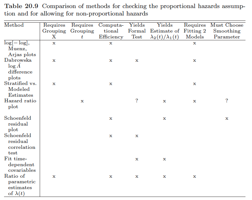
- graphic
- We may plot expected versus observed estimates of $S(t)$ to check if they are close.
- check parallelism of stratified log-log function, $\log[-\log S(t)]$, plots as $t \uparrow$
- We may use suitably defined residuals to test the goodness-of-fit.
- Consider eponymous residuals due to Schoenfeld (1982) that are centered on zero and should be independent of time if the PHA is true. Deviations from this, i.e. residuals that exhibit some trend in time, indicate that the PHA is violated. I.e., test of no correlation between the Schoenfeld residuals and (possibly rank) survival time.
- And we may generalize the model to be non-proportional and then assess whether the generalized model fits better than the proportional one.


-
The model
- Model specification
- baseline hazard is unspecified
-
Inference with partial likelihood
- Regression coefficients
-
Breslow estimator of the cumulative baseline hazard $$ \hat{\Lambda}_0(t|\hat{\beta}) = \int_0^t\frac{dN(u)}{\sum_iY_i(u)\exp(Z_i(u)^T\hat{\beta})} $$
- with no covariates ($\beta=0$) the Breslow estimator is simply the Nelson-Alen estimator.
-
The partial likelihood may be seen as a profile likelihood resulting from eliminating the baseline hazard from a joint likelihood including both $\beta$ and $\lambda_0(t)$.
-
It is important to notice that this joint likelihood is valid both for all-cause survival data (left panel of Figure 1) and for the more general situation depicted in the right panel of that figure. This is because the likelihood for the whole system factorizes into a number of factors, each depending on a separate transition in the model.

-
Internal vs external time-dependent covariates
- External (exogenous): time-dependent variables: can be calculated or they "exist" regardless the subject is still under observation or not. E.g. age
- Internal (endogenous): those can only be ascertained for subjects still under observation, e.g. current blood pressure
-
A limitation of this non-parametric model component is that it only allows direct estimation of the cumulative baseline hazard $Λ_0(t)$, but fails to produce an estimate of the hazard $𝜆_0(t)$ itself. To obtain an estimate of $𝜆_0(t)$ some smoothing would be required.
-
To allow greater flexibility and obtain a smooth baseline hazard one may use flexible parametric models for $𝜆_0(t)$, for example, via splines in combination with penalized likelihood.
Checklist when fitting the Cox model [1]
Before fitting the model
- Checks on the covariates to be included in the model
- Check dates
- Investigate censoring
- plotting a “survival curve” estimating $C(t) =P(\text{no censoring before } t)$ (or its complement $1 − C(t))$ could be done to give an impression of the proportion censored in time. Here, censoring is the “event” and a failure is a “censoring event” that prevents observation of the “event of interest.’
- a Cox regression model with “censoring” as event can help to check whether the censoring depends on any of the covariates under consideration.
- If there are some variables that one may or may not include in the model (maybe they are not crucial for the question asked) then they should be included if they affect the censoring, since in this way the independent censoring assumption is relaxed to conditional independence,
- An important feature of hazard models is that they can be used exactly by formally censoring for the competing events (including all-cause death).
- This is not a violation of the independent censoring assumption, the point being, as mentioned above, that the joint likelihood function for both the event of interest and the competing events factorizes and the factor corresponding to the intensity for the event of interest has the same form as it would have had if competing events were regarded as censoring events.
- In such situations one should carefully consider if the (cause-specific) hazard for the event of interest properly answers the scientific question or whether one needs to go beyond this hazard model.
- Time-dependent covariates
- A feature of the partial likelihood estimation method for the Cox model is that the values of time-dependent covariates are needed for everyone at risk at all the event times.
- In practice, most recently observed values of $Z(t)$ are typically carried forward until the next value is observed. Such last-value-carried-forward approach can induce some bias toward the null if the current hazard depends truly on the current (unknown) covariate value.
- A more advanced approach for internal time-dependent covari- ates which are not measured at all times uses joint longitudinal-survival models to obtain estimates of $\beta$, and also allows the possibility that the observed $Z(t)$ is measured with error.
- If the value of a time-dependent covariate at t captures the past history (Z(s), s < t) then issues of incomplete data may arise with delayed entry if (Z(s), s < V ) is not observed.
- Covariates that change shortly before the endpoint should be viewed with particular suspicion. e.g. change in medication in the last 1 or 2 weeks before death
- The most serious examples of such “anticipation” involve reverse causality bias where a change in Z(t) occurs because of early symptoms of the event of interest.
- A feature of the partial likelihood estimation method for the Cox model is that the values of time-dependent covariates are needed for everyone at risk at all the event times.
After fitting the model
- Check PH and the functional form
- Chekcing PH assumption
- Schoenfeld and martingale residuals
- Plots of the cumulative hazard
- through estimates of $\beta(t)$ in a time-varying coefficient Cox model
- For continuous covariates, functional form (ie, nonlinear effects) should ideally be investigated jointly with assessing possible violation of the PH hypothesis (ie, their “time-varying effects”)
- Note that violation of the PH assumption may be some times induced by a failure to include in the Cox model a strong predictor of the outcome.
- Chekcing PH assumption
- Reporting
- the regression parameters figuring in the partial likelihood only give information about the hazard ratios and the relevance and importance of the hazard ratios at any follow-up time depends on the concurrent values of the baseline hazard.
- Interpretation (hazard ratio)
- Noncollapsibility
- It is frequently seen that the effects, 𝛽, in a Cox model gradually decay with time toward 0.
- If the correct model is $\lambda(t) = \lambda_0(t)\exp(\beta_1Z_1+\beta_2Z_2)$ then a reduced model $\lambda(t)=\tilde{\lambda}_0\exp(\tilde{\beta}Z_1)$ cannot hold even if $Z_1$ and $Z_2$ are independent, so that $Z_2$ isn't considered a confounder for $Z_1$.
- The noncollapsibility suggests that PH can only be seen as a working hypothesis allowing a simple structure.
- It can be noted that the logistic regression model for a binary response variable suffers from the same problem, while the additive hazards model does not.
- It is frequently seen that the effects, 𝛽, in a Cox model gradually decay with time toward 0.
- Competing risk
- if individuals may die from causes other than the one of primary interest,no such direct interpretation in terms of probability of the event is possible. Directly using the conventional survial formula will over-estimate the probability of the event of interest.
- Instead, one should fit the Cox models for all transitions (cause-specific hazards) and interpret the collective results through study of the absolute risk (cumulative incidence function)
- Hazard ratios from cause-specific Cox models do no longer necessarily reflect the absolute risk ratio.
- Lack of causal interpretation
- the hazard does not provide a "causal contrast"
- The contrasts based on the hazard functions for the counterfactual outcomes $T^*(0), T^*(1)$, e.g. the hazard ratio at time $t$, are not directly causally interpretable since they contrast different subpopulations: those who survive past $t$ under treatment ($T^*(1)>t$) and those who survive past time $t$ under no treatment ($T^*(0)>t$).
- For this reason, a statement saying that“treatment only works until time 𝜏 but not beyond” in a situation with 𝛽(t) < 0 for t < 𝜏 and 𝛽(t) = 0 for t > 𝜏 is not justified.
- A special problem with causal inference for survival data is time-depending confounding/mediation where a time-dependent covariate both affects future treatment and survival outcome and is affected by past treatment. For this situation, special techniques are needed to draw causal conclusions concerning the treatment effect.
- the hazard does not provide a "causal contrast"
- Noncollapsibility
Alternatives/modifications to Cox PH model
-
Extended Cox model (with time-dependent coefficients when PH assumption doesn't hold)
$$\lambda(t, x) = \lambda_0(t)\exp(\beta_1X_1 + \sigma_1X_2g(t))$$
where $g(t)$ is a function of time, e.g. $t$, $log(t)$
-
The simplest example is to split time into two intervals (splitting at time 𝜏, say) and assume PH within each.
-
Alternatives include the use of splines. Some care is needed here since the number of parameters in such models with time-varying effects can become quite large and there is a danger of overfitting.
-
In the situation where the PH assumption needs to be relaxed for a single categorical covariate, the stratified Cox model is useful.
-
An alternative to the multiplicative PH models is an additive hazards model. The Aalen model
- both the baseline hazard $𝜆_0(t)$ and the regression functions $𝛽(t)$ are completely unspecified (like the baseline hazard for the Cox model) and their cumulatives $\int_0^t\lambda_0(u)du$, $\int_0^t\beta(u)du$ can be estimated using a least squares technique.
- A drawback of the Aalen model is that the estimated hazard can become negative while an advantage is that it is very flexible.
-
A completely different approach is given by the accelerated failure time (AFT) model where the covariates are assumed to extend or shorten the survival time by a constant time ratio $\exp(\beta)$
$$ S(t|Z) = S_0(\exp(-Z^T\beta)t) $$or equivalently
$$ \ln(T^*)= Z^T\beta + \epsilon $$- The model is a viable alternative to the PH model and although one could derive the hazard function for this model, it does not naturally fall under the heading of “hazard models.”
-
-
Ristricted mean survival time (RMST) model
Alternative HR [2]

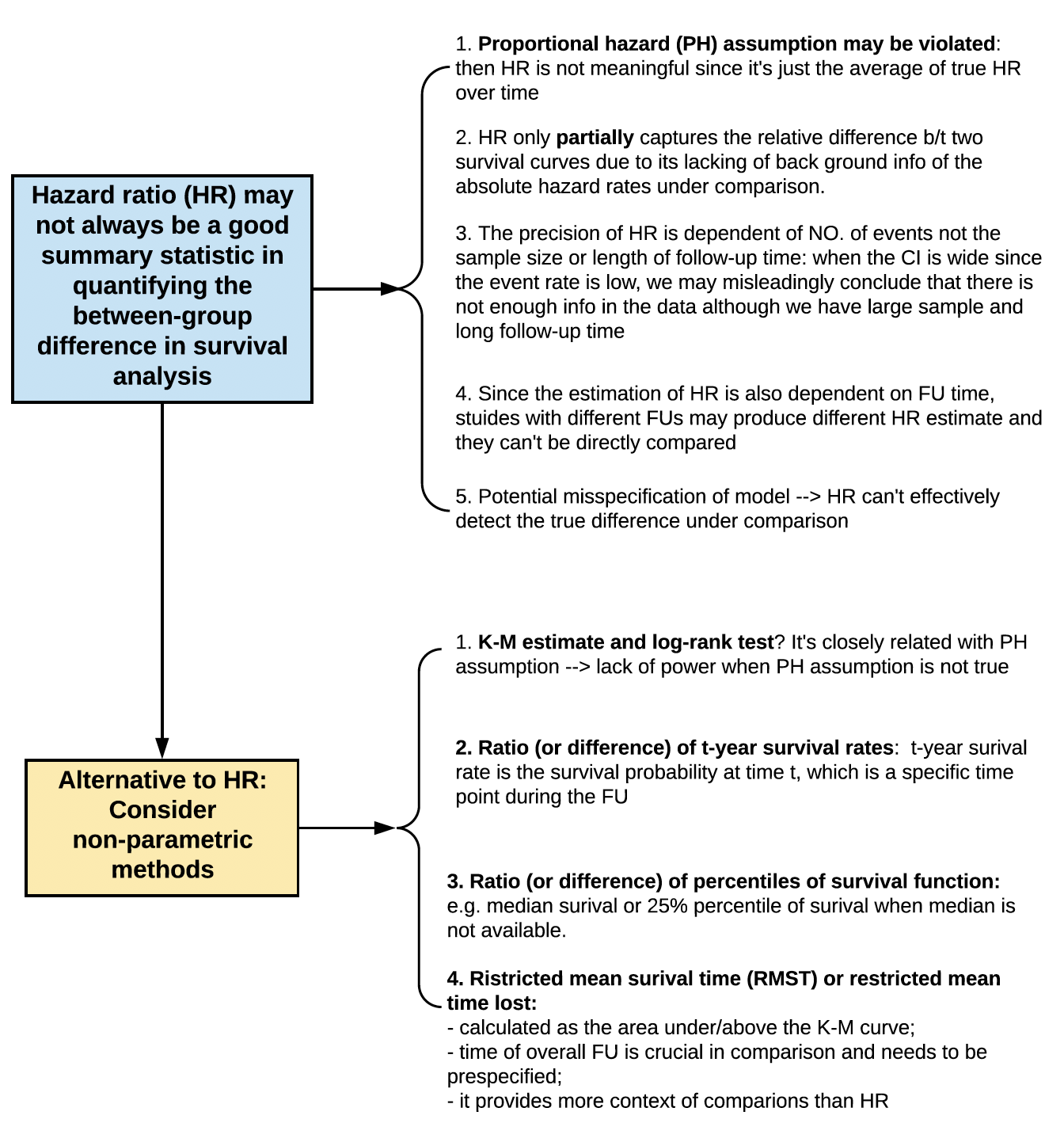
- Hazard ratio (HR) may not always be a good summary statistic in quantifying the between-group difference in survival analysis for the following reasons
- Proportional hazard (PH) assumption may be violated (see above): then HR is not meaningful since it's just the average of true HR over time
- HR only partially captures the relative difference b/t two survival curves due to its lacking of background info of the absolute hazard rates under comparison (?).
- The precision of HR is dependent of NO. of events not the sample size or length of follow-up time: when the CI is wide since the event rate is low, we may misleadingly conclude that there is not enough info in the data although we have large sample and long follow-up time
- Since the estimation of HR is also dependent on FU time, stuides with different FUs may produce different HR estimate and they can't be directly compared
- Potential misspecification of model $\rightarrow$ HR can't effectively detect the true difference under comparison
- Alternative to HR: consider non-parametric methods
- K-M estimate and log-rank test(?) It's closely related with PH assumption $\rightarrow$ lack of power when PH assumption is not true
- Ratio (or difference) of t-year survival rate: t-year survival rate is the survival probability at time $t$, which is a specific time point during the FU
- Ratio (or difference) of percentiles of survival function: e.g. median survival or 25% percentile of survival when median is not available
- Ristricted mean survival time (RMST) or restricted mean time lost
- Calculated as the area under/above the K-M curve
- time of overall FU is crucial in comparison and needs to be prespecified
- it provides more context of comparison than HR
References
Kragh Andersen, Per and Pohar Perme, Maja and van Houwelingen, Hans C and Cook, Richard J and Joly, Pierre and Martinussen, Torben and Taylor, Jeremy MG and Abrahamowicz, Michal and Therneau, Terry M (2021). Analysis of time-to-event for observational studies: Guidance to the use of intensity models. ↩︎
Uno, Hajime and Claggett, Brian and Tian, Lu and Inoue, Eisuke and Gallo, Paul and Miyata, Toshio and Schrag, Deborah and Takeuchi, Masahiro and Uyama, Yoshiaki and Zhao, Lihui and others (2014). Moving beyond the hazard ratio in quantifying the between-group difference in survival analysis. ↩︎