[book] Causal Inference: What If
by Miguel A. Hernan and James M. Robins
Chapter 2 Randomized Experiments
2.1 Randomization
- Counterfacatual: $Y^a$ the "theoretical" outcome under certain treatment $a$
-
Exchangeability assumption: $Y^a\perp\!\!\!\perp A$, the counterfacatual is independent of actual treatment assigned; i.e. the counterfacatual is "fixed" no matter what treatment the subject receives. It can be observed if the actual treatment received is the same as the counterfactual treatment.
-
Mean exchangeability: $E[Y^a|A=1] = E[Y^a|A=0] \text{ for all } a$
- Exchangeability implies mean exchangeability, but not verse vasa (e.g. due to the difference in other distributional parameter, such as variance)
- For dichotomous outcomes, exchangeability is equivalent to mean exchangeability
-
In ideal randomized experiments association is causation.
2.2 Conditional randomization
-
Conditionally randomized experiments meaning there are several randomization probabilities that depend (are conditional) on the values of some variable(s) $L$.
-
Marginally randomized experiments meaning there is only a single unconditional (marginal) randomization probability (doesn't need to be 0.5) that is common to all individuals.
- a marginally randomized experiment is expected to result in exchangeability of the treated and the untreated:
-
In contrast, a conditionally randomized experiment will not generally result in exchangeability of the treated and the untreated because, by design, each group may have a different proportion of individuals with bad prognosis.
-
However, the conditional (or stratified) randomization can be considered as a combination of separate marginal randomiztions from each unique stratum defined by the randomization factors, within which the general rules of marginal randomization and causal inference apply, that is
$$ Pr[Y^a=1|A =1, L=l]=Pr[Y^a=1|A =0, L=l] \text{ or } Y^a \perp\!\!\!\perp A|L=l \text{ for all } a $$ -
To calculate the population average causal effect with conditional randomization, do the following two steps
- First, compute the average causal effect in each of these subsets or strata of the population
- Second, compute the average causal effect by combining the individual effects from step 1
- Using standardization or inverse probability weighting (wich are mathmatically equivalent)
2.3 Standardization
-
More formally, in standardization, the marginal counterfactual risk $Pr[Y^a=1]$ is the weighted average of the stratum-specific risks $Pr[Y^a=1|L=0]$ and $Pr[Y^a=1|L=1]$ with weights equal to the proportion of individuals in the population with $L=0$ and $L=1$, respectively.
-
Derivation of counterfactual risk by standardization
$$ Pr(Y^a=1) = \sum_l Pr(Y^a=1|L=l)Pr(L=l) $$under conditoinal exchangeability, we can replace the (unobserved) counterfactual riks with the obsered risk:
$$ Pr(Y^a=1|L=l) = Pr(Y=1|A=a, L=l) $$- When, as here, a counterfactual quantity can be expressed as function of the distribution (i.e., probabilities) of the observed data, we say that the counterfactual quantity is identified or identifiable; otherwise, we say it is unidentified or not identifiable.
2.4 Inverse probability weighting (IPW)
-
Under conditional exchangeability $Y^a \perp\!\!\!\perp A|L$ in the original population, the treated and the untreated are (unconditionally) exchangeable in the pseudo-population because the $L$ is independent of $A$.
- That is, the associational risk ratio in the pseudo-population is equal to the causal risk ratio in both the pseudo-population and the original population.
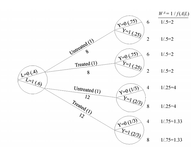
-
Informally, the pseudo-population is created by weighting each individual in the population by the inverse of the conditional probability of receiving the treatment level, IP weight:
$$ W^A = 1/f(A|L) $$ -
Standardization and IP weighting are mathematically equivalent
- In fact, both standardization and IP weighting can be viewed as procedures to build a new tree in which all individuals receive treatment $a$. Each method uses a different set of the probabilities to build the counterfactual tree: IP weighting uses the conditional probability of treatment $A$ given the covariate $L$ (as shown in Figure above), standardization uses the probability of the covariate $L$ and the conditional probability of outcome $Y$ given $A$ and $L$.
- Because both standardization and IP weighting simulate what would have been observed if the variable (or variables in the vector) $L$ had not been used to decide the probability of treatment, we often say that these methods adjust for $L$.
-
Proof of the equivalence of IP weighting and standardization
-
Standardized mean for treatment level $a$ is defined as
$$ \sum_l E\left[Y|A=a, L=l\right]Pr(L=l) $$ -
IP weighted mean for the treatment level $a$ is defined as
$$ E\left[\frac{I(A=a)Y}{f(A|L)}\right] $$- proof of equivalence
-
-
It can be shown that both estimates of mean are euqal to the counterfactual mean $E[Y^a]$ under the conditional exchangeability assumption, that is
$$ E[Y^a] = \sum_l E\left[Y|A=a, L=l\right] = E\left[\frac{I(A=a)Y}{f(A|L)}\right], \text{ under } Y\perp\!\!\!\perp A|L $$- When treatment is continuous, which is an unlikely design choice in conditionally randomized experiments, $E[I(A=a)Y/f(A|L)]$ is no longer equal to $\sum_l E\left[Y|A=a, L=l\right]$ and thus is biased for $E[Y^a]$ even under exchangeability
Chapter 4 Effect Modification
- Key ideas in this chapter
- Definition of effect modification (EM); why we care about it?
- How to identify/quantify effect modification? Hint: use stratification
- Stratification and matching are both adjustment methods; what is the definition of adjustment? Any other adjustment methods?
4.1 & 4.3 Definitionof effect modification (what) and why effect modification
-
Definition of effect modification
- We say that $V$ is a modifier of the effect of $A$ on $Y$ when the average causal effect of $A$ on $Y$ varies across levels of $V$
- The existence of effect modification depends on the effect measure being used (e.g., risk difference, risk ratio), so it is more accurate to use the term effect-measure modification, to emphasize the dependence of the concept on the choice of effect measure
- Since the average causal effect can be measured using different effect measures (e.g., risk difference, risk ratio), the presence of effect modification depends on the effect measure being used.
- Here only consider variables $V$ that are not affected by treatment $A$
- We say that $V$ is a modifier of the effect of $A$ on $Y$ when the average causal effect of $A$ on $Y$ varies across levels of $V$
-
Types of effect modification
- qualitative effect modification: when the average causal effects in the subsets are in the opposite direction.
- In the presence of qualitative effect modification, additive effect modification implies multiplicative effect modification, and vice versa. In the absence of qualitative effect modification, however, one can find effect modification on one scale (e.g., multiplicative) but not on the other (e.g., additive).
- qualitative effect modification: when the average causal effects in the subsets are in the opposite direction.
-
Why we care about effect modification
- If a factor $V$ modifies the effect of treatment $A$ on the outcome $Y$ then the average causal effect will differ between populations with different prevalence of $V$
- There is generally no such athingas “the average causal effect of treatment $A$ on outcome $Y$ (period)”, but “the average causal effect of treatment $A$ on outcome $Y$ in a population with a particular mix of causal effect modifiers.”
- Evaluating the presence of effect modification is helpful to identify the groups of individuals that would benefit most from an intervention.
- if there is a nonzero causal effect in at least one stratum of $V$ and the counterfactual risk $Pr[Y^{a=0} =1|V = v]$ varies with $v$,then effect modification is guaranteed on either the additive or the multiplicative scale.
- Additive, but not multiplicative, effect modification is the appropriate scale to identify the groups that will benefit most from intervention.
- The identification of effect modification may help understand the biological, social, or other mechanisms leading to the outcome.
- If a factor $V$ modifies the effect of treatment $A$ on the outcome $Y$ then the average causal effect will differ between populations with different prevalence of $V$
-
Transportability of causal inference: The extrapolation of causal effects computed in one population to a second population
- Conditional causal effects in the strata defined by the effect modifiers may be more transportable than the causal effect in the entire population, but there is no guarantee that the conditional effect measures in one population equal the conditional effect measures in another population. Due to different reasons:
- unmeasured, or unknown, causal effect modifiers whose conditional distributions vary between the two populations
- when transportability may be justified from one to antoher population?
- Effection modification: similar distribution of effect modifiers
- Versions fo treatment: requires similar distr. of versions fo treatment
- Interference: treating one individual many affect the outcome of others in the populaiton
- transportability of causal effects is an unverifiable assumption that relies heavily on subject-matter knowledge. It is a more difficult problem than the identification of causal effects in a single population
- Conditional causal effects in the strata defined by the effect modifiers may be more transportable than the causal effect in the entire population, but there is no guarantee that the conditional effect measures in one population equal the conditional effect measures in another population. Due to different reasons:
4.2, 4.4, & 4.5 How to quantify effect modification
Stratification
- To identify effect modification by $V$ in an ideal experiment with unconditional randomization, one just needs to conduct a stratified analysis, that is, to compute the association measure in each level of the variable $V$.
- The procedure to compute the conditional risks $Pr[Y^{a=1}=1|V = v]$ and $Pr[Y^{a=0}=1|V = v]$ in each stratum $v$ has two stages: 1) stratification by $V$ , and 2) standardization by $L$ (or, equivalently, IP weighting with weights depending on $L$).
Adjustment via stratification
-
In practice stratification is often used as an alternative to standardization (and IP weighting) to adjust for $L$. In fact, the use of stratification as a method to adjust for $L$ is so widespread that many investigators consider the terms “stratification” and “adjustment” as synonymous.
- Stratification provides conditional effect measures within each of the stratum
-
Unlike standardization and IP weighting, adjustment via stratification requires computing the effect measures in subsets of the population defined by a combination of all variables $L$ that are required for conditional exchangeability.
- That is, the use of stratification forces one to evaluate effect modification by all variables $L$ required to achieve conditional exchangeability, regardless of whether one is interested in such effect modification.
-
Other problems associated with the use of stratification are noncollapsibility of certain effect measures like the odds ratio (Fine Point 4.3) and inappropriate adjustment that leads to bias when, in the case for time-varying treatments, it is necessary to adjust for time-varying variables $L$ that are affected by prior treatment (see Part III of the book).
- Ristriction: compute causal effect in only some of the strata defined by the variables $L$ and no stratum-specific measures for some other strata
Adjustment via matching
-
The goal of matching is to construct a subset of the population in which the variables $L$ have the same distribution in both the treated and the untreated.
- Under the assumption of conditional exchangeability given $L$, the result of this procedure is (unconditional) exchangeability of the treated and the untreated in the matched population.
- The chosen group defines the subpopulation on which the causal effect is being computed (e.g. effect in the treated/untreated)
-
Because the matched population is a subset of the original study population, the distribution of causal effect modifiers in the matched study population will generally differ from that in the original, unmatched study population
Fine and Tech Points 4.1 Causal effect in the treated/untreated
- Consider a particular and special subset of the population, the treated ($A=1$), the average causal effect in the treated is expressed as
- The causal risk ratio in the treated is also called the standardized morbidity ratio (SMR)
- The average effect in the treated will differ from the average effect in the population if the distribution of individual causal effects varies between the treated and the untreated.
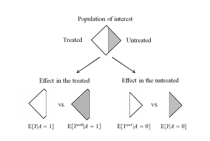
-
Computing the average causal effect in the treated only requires partial exchangeability $Y^{A=0} \perp\!\!\!\perp A|L$.
- similarly, the average causal effect in the untreated is computed under the partial exchangeability condition $Y^{a=1} \perp\!\!\!\perp A|L$
-
To compute the counterfactual mean $E(Y^{a}|A=a')$:
-
Standardization
$$ E(Y^{a}|A=a') = \sum_l E(Y|A=a, L=l)Pr(L=l|A=a') $$ -
IP weighting
$$ E(Y^{a}|A=a') = \frac{E\left[\frac{I(A=a)Y}{f(A|L)Pr(A=a'|L)}\right]}{E\left[\frac{I(A=a)}{f(A|L)Pr(A=a'|L)}\right]} $$
-
4.6 Summary
-
Stratified analysis is needed to inspect the existence of effect modification from certain variable(s) $L$ on the treatment $A$
-
When doing standardization and IP weighting, stratefication is used as a technique to estimate the average/weighted outcome in each of the treatment arms to construct the final estimate of the treatment effect
$$ \begin{array}{ll} Pr(Y^{a=1}=1) - Pr(Y^{a=0}=1) &= \sum_lPr(Y^{a=1}=1|L=l) - \sum_lPr(Y^{a=0}=1|L=l) \\ &= \sum_l Pr(Y=1|A=1, L=l) - \sum_l Pr(Y=1|A=0, L=l) \end{array} $$ -
In contrast, pooling stratum-specific effect (e.g., Woolf, Mantel-Haenszel, maximum likelihood) needs to compute the stratum-specific effect first followed by combining the individual effects using some kind of weighted average with weights chosen to reduce the variability of the pooled estimate.
- The main goal of pooling is to obtain a narrower confidence interval around the common stratum-specificeffect measure, but the pooled effect measure is still a conditional effect measure.
-
These four approaches can be divided into two groups according to the type of effect they estimate: standardization and IP weighting can be used to compute either marginal or conditional effects, stratification/restriction and matching can only be used to compute conditional effects in certain subsets of the population.
- The idea is that, if the effect measure is the same in all strata (i.e., if there is no effect-measure modification), then the pooled effect measure will be a more precise estimate of the common effect measure.
- In the absence of effect modification, the effect measures (risk ratio or risk difference) computed via standardization, IP weighting, stratification/restriction, and matching will be equal.
-
Investigators conducting observational studies need to explicitly define the causal effect of interest and the subset of the population in which the effect is being computed. Otherwise, misunderstandings might easily arise when effect measures obtained via different methods are different.
Chapter 5 Interaction
- Key ideas/points in this chapter
- What is an interaction?
- What is the difference between interaction and effect modification?
- How is an interaction caused? How to identify it?
- What is sufficient causes and sufficient cause interaction? How is sufficient component causes related with counterfactual response types? (optional)
5.1 Interaction requires a joint intervention
-
Joint interventions: interventions on two or more treatments
-
Definition of interaction:
- There is interaction between two treatments $A$ and $E$ if the causal effect of $A$ on $Y$ after a joint intervention that set $E$ to 1 differs from the causal effect of $A$ on $Y$ after a joint intervention that set $E$ to 0.
- Depending on the choice of effect measure, the interaction can be on the additive scale or multiplicative scale
-
Differentiating interaction and effect modification
- Under interaction, there are two treatments, and these two treatments have euqal status in the definition of interaction. That is the counterfactual can be defined on either interventions to define the existence of interaction
- In contrast, the definition of effect modification involves the counterfactual outcomes only on one of the two variables, i.e. the treatment variable of interest (say, $Y^a$) but not the counterfactual outcomes $Y^{a, v}$.
5.2 Identifying interaction
-
Identifying interaction requires exchangeability, positivity, and consistency for both treatments.
- When both treatments are randomly assigned, then the concepts of interaction and effect modification conincide.
and the techniques used to identify effect modification can be used to identify interaction.
- When one of the treatment, say $E$, is not randomly assigned, four marginal risks $Pr(Y^{a, e} = 1)$ need to be computed under the usual identifying assumtpions, by standardiztion or IP weighting conditional on the measured covariates.
- Rather than viewing $A$ and $E$ as two distinct treatments with two possible levels (1 or 0) each, one can view $AE$ as a combined treatment with four possible levels (11, 01, 10, 00) and interaction can be evaluated when exchangeability, positivity,and consistency are all satisfied for the joint treatment $(A, E)$.
- However, this condistion is not necessary when the two tretments occur at different times (see Part III of the book)
- Rather than viewing $A$ and $E$ as two distinct treatments with two possible levels (1 or 0) each, one can view $AE$ as a combined treatment with four possible levels (11, 01, 10, 00) and interaction can be evaluated when exchangeability, positivity,and consistency are all satisfied for the joint treatment $(A, E)$.
-
When conditional exchangeability can only be assumed for treatment $A$ but $E$, one cannot generally assess the presence of interaction between $A$ and $E$, but can still assess the presence of the effect modification by $E$.
- Thus, there can be modification of the effect of $A$ by another variable without interaction between $A$ and that variable.
5.3 Counterfactual response types and interaction
-
Each combination of counterfactual responses is often referred to as are sponse pattern or a response type.
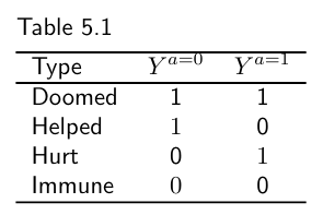
-
When considering two dichotomous treatments $A$ and $E$,thereare16 possible response types because each individual has four counterfactual outcomes
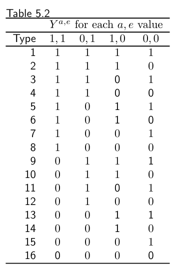
-
if all individuals in the population have response types 1, 4, 6, 11, 13 and 16 then there will be no interaction between $A$ and $E$ on the additive scale.
-
The presence of additive interaction between $A$ and $E$ implies that, for some individuals in the population, the value of their two counterfactual outcomes under $A = a$ cannot be determined without knowledge of the value of $E$, and vice versa.
- types 8, 12, 14, and 15
- types 7 and 10
- types 2, 3, 5, and 9
-
-
5.4 Sufficient causes & 5.5 Sufficient causes interaction & 5.6
-
We refer to the smallest set of background factors that, together with $A =1$ are sufficient to inevitably produce the outcome as $U_1$. The simultaneous presence of treatment $(A=1)$ and $U_1=1$ is a minimal sufficient cause of the outcome $Y$.
- By definition of background factors, the dichotomous variables $U$ cannot be intervened on, and cannot be affected by treatment $A$.
- The term sufficient-component causes is often used to refer to the sufficient causes and their components (e.g. $A$ or $U$ or both).
-
The definition of interaction within the counterfactual framework does not require any knowledge about those mechanisms nor even that the treatments work together (see Fine Point 5.3).
-
A sufficient cause interaction between $A$ and $E$ exists in the population if $A$ and $E$ occur together in a sufficient cause.
- Synergistic: when $A=1$ and $E=1$ are present in the same sufficient cause
- Antagonistic: when $A=1$ and $E=0$ (or $A=0$ and $E=1$) are present in the same sufficient cause
-
The correspondence between conterfactual response types and the sufficient component causes
-
Example with a dichtomous treatment and outcome

-
A particular combination of component causes corresponds to one and only one counterfactual type.
-
However, a particular response type may correspond to several combinations of component causes
-
There will be exchangeability if the proportions of “doomed” + “hurt” ($U_0=1$ or $U_1=1$) and of “doomed” + “helped” ($U_0=1$ or $U_1=2$) are equal in the treated and the untreated. That is, exchangeability for a dichotomous treatment and out come can be expressed in terms of sufficient-component causes as
$$ Pr(U_0=1 \text{ or } U_1=1|A=1) = Pr(U_0=1 \text{ or } U_1=1|A=0), \text{ and} $$$$ Pr(U_0=1 \text{ or } U_2=1|A=1) = Pr(U_0=1 \text{ or } U_2=1|A=0) $$
-
-
In epidemiologic discussions, sufficient cause interaction is commonly referred to as biologic interaction (Rothman et al, 1980).
-
Counterfactuals or sufficient-component causes
-
The sufficient component cause model considers sets of actions, events, or states of nature which together inevitably bring about the outcome under consideration.
- It addresses the question, “Given a particular effect, what are the various events which might have been its cause?”
-
The potential outcomes or counterfactual model focuses on one particular cause or intervention and gives an account of the various effects of that cause.
- the potential outcomes framework addresses the question, “What would have occurred if a particular factor were intervened upon and thus set to a different level than it in fact was?”
-
The counterfactual approach addresses the question “what happens?” The sufficient-component-cause approach addresses the question “how does it happen?”
-
Though the sufficient-component-cause framework is useful from a pedagogic standpoint, its relevance to actual data analysis is yet to be determined.
-
Suffcient-component-cause framework's conclusions depend on the coding on the outcome, and is by definition limited to dichotomous treatments and outcomes (or to variables that can be recoded as dichotomous variables).
-
Some apparently alternative frameworks–causal diagrams, decision theory–are essentially equivalent to the counterfactual framework
-
Chapter 6 Graphical representation of causal effects
- Key ideas/points in this chapter
- What is a DAG (Direct Acyclic Graph), what is it used for? (6.1)
- DAG representation of the key causal inference concepts: marginal/conditional independence, positivity, and consistency (Section 6.2 to 6.4)
- D-seperation (6.4)
- Faithfullness (6.4)
- Type of biases (6.5)
- DAG representation of effect modification (6.6)
6.1 Causal diagrams
-
Causal diagrams like the one below are known as directed acyclic graphs, which is commonly abbreviated as DAGs.

-
The presence of an arrow pointing from a particular variable $V$ to another variable $W$ indicates that we know there is a direct causal effect (i.e., an effect not mediated through any other variables on the graph) for at least one individual.
-
In DAG, the variable $V_m$ is a descendant of $V_j$ (and $V_j$ is an ancestor of $V_m$) if there is a sequence of nodes connected by edges between $V_j$ and $V_m$ such that, following the direction indicated by the arrows, one can reach $V_m$ by starting at $V_j$.
-
A causal DAG is a DAG in which
- the lack of an arrow from node $V_j$ to $V_m$ (i.e., $V_j$ is not a parent of $V_m$)can be interpreted as the absence of a direct causal effect of $V_j$ on $V_m$ relative to the other variables on the graph,
- all common causes, even if unmeasured, of any pair of variables on the graph are themselves on the graph, and
- any variable is a cause of its descendants.
-
-
A defining property of causal DAGs is that, conditional on its direct causes, any variable on the DAG is independent of any other variable for which it is not a cause.
- This assumption, referred to as the causal Markov assumption, implies that in a causal DAG the common causes of any pair of variables in the graph must be also in the graph.
-
Conventional causal diagrams do not include the underlying counterfactual variables on the graph. Therefore the link between graphs and counterfactuals has traditionally remained hidden.
- The Single World Intervention Graph (SWIG)–seamlessly unifies the counterfactual and graphical approaches to causal inference by explicitly including the counterfactual variables on the graph.
6.2-6.4 Causal diagrams and marginal independence, conditional independence, positivity and consistency
-
Two variables are (marginally) associated if one causes the other, or if they share common causes. Otherwise they will be (marginally) independent ($A$ and $L$ in Figure 6.4 below).

- The common effect $L$ is referred to as a collider on the path $A \rightarrow L \leftarrow Y$ because two arrowheads collide on this node.
-
Association, unlike causation, is a symmetric relationship between two variables; thus, when present, association flows between two variables regardless of the direction of the causal arrows.
- In Figure 6.3 below, $A$ and $Y$ are associated because there is a flow of association from $A$ to $Y$ (or, equivalently, from $Y$ to $A$) through the common cause $L$.
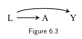
- In Figure 6.3 below, $A$ and $Y$ are associated because there is a flow of association from $A$ to $Y$ (or, equivalently, from $Y$ to $A$) through the common cause $L$.
-
When conditional independence is established
-
Effect of $A$ on the outcome $Y$ is only through a mediator $B$, and the analysis is conditonal on $B$: $A\perp\!\!\!\perp Y|B$

-
Conditioning on the common cause of $A$ and $Y$ (outcome): $A\perp\!\!\!\perp Y|L$
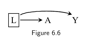
- Blocking the flow of association between treatment and outcome through the common cause is the graph-based justification to use stratification as a method to achieve exchangeability.
-
-
When conditional association is introduced
-
Conditional on the collider or its consequence, the common causes of the the collider (the outcome) are then associated/not independent any more
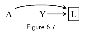
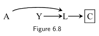
- Causal graphs theory shows that indeed conditioning on a collider like $L$ opens the path $A\rightarrow L \leftarrow Y$ ,which was blocked when the collider was not conditioned on.
- Causal graphs theory shows that conditioning on a variable $C$ affected by a collider $L$ also opens the path $A\rightarrow L \leftarrow Y$. This path is blocked in the absence of conditioning on either the collider $L$ or its consequence $C$.
-
-
Three structural reasons why two variables may be associated:
- one causes the other,
- they share common causes, or
- they share a common effect and the analysis is restricted to certain level of that common effect (or of its descendants).
- There is another possible source of association between two variables that we have not discussed yet: chance or random variability.
-
Standardization and IP weighting can also be derived using causal graphs theory, as part of what is sometimes referred to as the do-calculus.
-
"D-seperation": to define a path to be either blocked or open
- If there are no variables being conditioned on, a path is blocked if and only if two arrowheads on the path collide at some variable on the path.
- Any path that contains a non-collider that has been conditioned on is blocked.
- A collider that has been conditioned on does not block a path.
- A collider that has a descendant that has been conditioned on does not block a path.
- Two variables are d-separated if all paths between them are blocked (otherwise they are d-connected).
- Two sets of variables are d-separated if each variable in the first set is d-separated from every variable in the second set.
- The relationship between statistical independence and the purely graphical concept of d-separation relies on the causal Markov assumption (Technical Point 6.1):
- In a causal DAG, any variable is independent of its non-descendants conditional on its parents.
- The causal Markov assumption implies that, given any three disjoint sets $A$, $B$, $C$ of variables, if $A$ is d-separated from $B$ conditional on $C$,then $A$ is statistically independent of $B$ given $C$.
- The assumption that the converse holds, i.e., that $A$ is d-separated from $B$ conditional on $C$ if $A$ is statistically independent of $B$ given $C$, is a separate assumption–the faithfulness assumption described in Fine Point 6.2.
-
Positivity
- Positivity is roughly translated into graph language as the condition that the arrows from the nodes $L$ to the treatment node $A$ are not deterministic.
-
Consistency
- The first component of consistency–well-defined interventions–means that the arrow from treatment $A$ to outcome $L$ corresponds to a possibly hypothetical but relatively unambiguous intervention.
-
Positivity is concerned with arrows into the treatment nodes, and well-defined interventions are only concerned with arrows leaving the treatment nodes.
-
Faithfullness
-
Formally, faithfulness is the assumption that, for three disjoint sets $A$, $B$, $C$ on a causal DAG, (where $C$ may be the empty set), $A$ independent of $B$ given $C$ implies $A$ is d-separated from $B$ given $C$.
-
When the causal diagram makes us expect a non-null association that does not actually exist in the data (e.g. due to effect modification, which is rare ), we say that the joint distribution of the data is not faithful to the causal DAG.
-
In some occassions, faithfulness may be violated by design: for example in mathcing
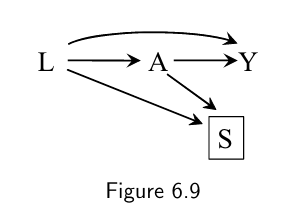
- selection $S$ (1: yes, 0: no) is determined by both $L$ and $A$. The box around $S$ indicates that the analysis is restricted to those selected into the matched cohort ($S$ =1)
- there are two open paths between $A$ and $L$ when conditioning on $S$: $L \rightarrow A$ and $L \rightarrow S \leftarrow A$ thus association between $A$ and $S$ are expected.
- However, matching creates an association via the path $L \rightarrow S \leftarrow A$ that is of equal magnitude, but opposite direction, as the association via the path $L \rightarrow A$. The net result is a perfect cancellation of the associations and matching leads to unfaithfulness.
-
Faithfulness may be violated when there exist deterministic relations between variables on the graph.
-
6.5 A structural classification of bias
-
We say that there is systematic bias when the data are insufficient to identify–compute–the causal effect even with an infinite sample size.
- Informally, we often refer to systematic bias as any structural association between treatment and outcome that does not arise from the causal effect of treatment on outcome in the population of interest
-
For the average causal effect in the entire population, we say that there is (unconditional) bias when $Pr[Y^{a=1} =1]− Pr[Y^{a=0}=1]=Pr[Y =1|A =1]− Pr [Y =1|A =0]$, which is the case when (unconditional) exchangeability $Y^{a} \perp\!\!\!\perp A$ does not hold.
- For the average causal effects within levels of $L$, we say that there is conditional bias whenever $Pr[Y^{a=1}=1|L = l] − Pr[Y^{a=0}=1|L = l]$ differs from $Pr[Y =1|L=l, A =1]− Pr [Y =1|L=l, A =0]$ for at least one stratum $l$, which is generally the case when conditonal exchangeability $Y^{a} \perp\!\!\!\perp A|L=l$ doesn not hold for all $a$ and $l$.
-
Absence of (unconditional) bias implies that the association measure (e.g., associational risk ratio or difference) in the population is a consistent estimate of the corresponding effect measure (e.g., causal risk ratio or difference) in the population.
The following three chapters (7, 8, 9) are about different sources of biases in causal analysis, which are
- Confounding: common cause of intervention and outcome
- Selection bias: common effect
- Measurement bias or information bias
6.6 The structure of effect modification
-
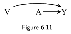
The causal diagram in Figure 6.11 includes the effect modifier $V$ with an arrow into the outcome $Y$ but no arrow into treatment $A$ (which is randomly assigned and thus independent of $V$).
- First, the causal diagram in Figure 6.11 would still be a valid causal diagram if it did not include $V$ because $V$ is not a common cause of $A$ and $Y$. It is only because the causal question makes reference to $V$ (i.e., what is the average causal effect of $A$ on $Y$ within levels of $V$?), that $V$ needs to be included on the causal diagram.
- Second, the causal diagram in Figure 6.11 does not necessarily indicate the presence of effect modification by $V$.
-
Many effect modifiers, however, do not have a causal effect on the outcome. Rather, they are surrogates for variables that have a causal effect on the outcome.
-
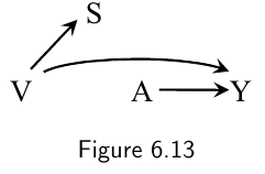
Ananalys is stratified by $S$ (but not by $V$) will generally detect effect modification by $S$ even though the variable that truly modifies the effect of $A$ on $Y$ is $V$.
- The variable $S$ is a surrogate effect modifier where as the variable $V$ is a causal effect modifier
- A surrogate effect modifier is simply a variable associated with the causal effect modifier.
- Because causal and surrogate effect modifiers are often indistinguishable in practice, the concept of effect modification comprises both.
- The variable $S$ is a surrogate effect modifier where as the variable $V$ is a causal effect modifier
-
surrogate effect modifiers can be associated with the causal effect modifier by structures including common causes, conditioning on common effects, or cause and effect.
-
Chapter 7 Confounding
- Key ideas/points in this chapter
- Defintion of confounding and confounder (7.3 & 7.4)
- What are the issues with the traditional defintion of confounder? why doesn't it work? And how to fix them?
- What are the common types of confoundings? (7.1)
- What is the back door criterion (and the front door fomula)? (7.3, 7.6)
- How to adjust for confounding?
- What is the Single-world intervention graph (SWIG)? (7.5)
- Defintion of confounding and confounder (7.3 & 7.4)
Confounding and confounders (7.1 & 7.4)
- Confounding (7.1)
-
The bias caused by shared causes of treatment and outcome
- The structure of confounding can be represented by using causal diagrams, i.e. when there is a backdoor path exists
-
-
(7.4) Under the traditional approach, a confounder was defined as a variable that meets the following three conditions:
- (1) it is associated with the treatment,
- (2) it is associated with the outcome conditional on the treatment (with “conditional on the treatment” often replaced by “in the untreated”), and
- (3) it does not lie on a causal pathway between treatment and outcome.
-
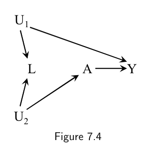
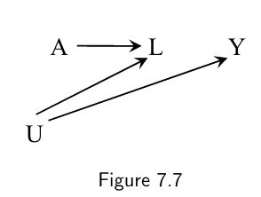
An approach based on a definition of confounder (i.e. the traditional approach) that relies almost exclusively on statistical considerations may lead, as shown by Figures 7.4 and 7.7, to the wrong advice: adjust for a “confounder” even when structural confounding does not exist.
- The problem arises because the traditional approach starts by defining confounders in the absence of sufficient causal knowledge about the sources of confounding, and then mandates adjustment for those so-called confounders.
-
Fixing the traditional definition of confounder:
- Replace condition (3) by the condition that “there exist variables $L$ and $U$ such that there is conditional exchangeability within their joint levels $Y^a \perp\!\!\!\perp A|L, U$.
- Replace conditions (1) and (2) by the following condition: $U$ can be decomposed into two disjoint subsets $U_1$ and $U_2$ (i.e., $U=U_1\cup U_2$ and $U=U_1\cap U_2$ is empty) such that (i) $U_1$ and $A$ are not associated within strata of $L$, and (ii) $U_2$ and $A$ are not associated within joint strata of $A$, $L$, and $U_1$.The variables in $U_1$ may be associated with the variables in $U_2$. $U_1$ can always be chosen to be the largest subset of $U$ that is unassociated with treatment.
-
In contrast, a structural approach starts by explicitly identifying the sources of confounding–the common causes of treatment and outcome that, were they all measured, would be sufficient to adjust for confounding–and then identifies a sufficient set of adjustment variables.
- The structural approach makes clear that including a particular variable in a sufficient set depends on the variables already included in the set.
- Given a causal DAG, confounding is an absolute concept whereas confounder is a relative one.
-
the structural approach to confounding has two important advantages.
- First, it prevents inconsistencies between beliefs and actions.
- Second, the researchers’ assumptions about confounding become explicit and therefore can be explicitly criticized by other investigators.
The structure (type) of confounding (7.1)
- Healthy worker bias: e.g. the effect of working as a firefighter on the risk of death will be confounded if "being physically fit" is a cause of both being an active firefighter and having a lower mortality rate.
- Confounding by indication or channeling: e.g. the effect of drug on teh risk of disease will be confounded if the drug is more likely to be prescribed to individuals with certain condition that is both an indication for treatment and a risk factor for the disease.
- Reverse causation: e.g. the effect of behavior on the risk of death will be confounded if the behavior is associated with another behavior that has a causal effect on death and tends to co-occur with the behavior.
- Linkage disequilibrium or population stratification: e.g. the effect of a DNA sequence on the risk of developing certain trait will be confounded if there exists another DNA sequence that has a causal effect on y and is more frequent among people carrying the first DNA sequence.
Confounding and exchangeability (7.2), Backdoor criterion (7.3) & front door criterion (7.6)
-
The presence of common causes of treatment and outcome causes confounding because it creates an open backdoor path
-
A open backdoor path can be block by conditioning on a variable on the path
-
A backdoor path is blocked if there is a collider on the path; conditioning on the collider opens the backdoor path
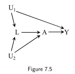
- The definition of collider is pathspecific: $L$ is a collider on the path $A\leftarrow U_2 \rightarrow L \leftarrow U_1 \rightarrow Y$ , but not on the path $A \leftarrow L \leftarrow U_1 \rightarrow Y$.
- conditioning on a collider, which happens to be a common effect, may open a previously blocked backdoor path and introduces selection bias.
-
In Figure 7.5, the bias is intractable: attempting to block the confounding path opens a selection bias path. There is neither unconditional exchangeability nor conditional exchangeability given $L$.
-
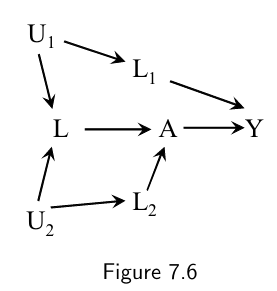
A solution to the bias in Figure 7.5 would be to measure either (i) a variable $L_1$ between $U_1$ and either $L$ or $Y$ (condition on $L_1$ is adequate), or (ii) a variable $L_2$ between $U_2$ and either $L$ or $A$ (condition on both $L_2$ and $L$).
-
-
The front door formula
-
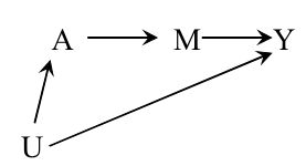
Given the following DAG, where U is an unobserved confounder, the average causal effect of A on Y cannot be idenfitied with the standardization or IP weighting methods to compurate the counterfactual risk $Pr(Y^a=1)$.
-
- Instead, the so-called front door formula can be used to calculate the counterfactual
Single-world intervention graphs (7.5)
Confounding adjustment (7.6)
Chapter 8 Selection bias
- Source/structure (type of) selection bias
- Selection bias vs confounding and censoring
- How to adjust selection bias
- How to avoid selection bias